1. Introduction
import numpy as np
import matplotlib.pyplot as plt
import pandas as pd
%matplotlib inline
The Logistic Regression uses the the logistic function to restrict predicted values from 0 to 1. It is also called the sigmoid function. It is S-shaped and assign any real-valued number to a value between 0 and 1. It is worth noting 0 and 1 are excluded e.g ]0, 1[.
It is defined as below :
$g(x)=\frac{1}{1 + e^{-x}}$
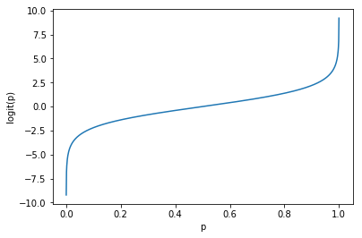
To understand where this expression comes from, let’s work with odds. Odds are linked to probabilities by this formula : $odds = \frac{p}{1-p}$ where p is the probability.
Taking the natural logarithm of odd lead us to build logit function : $ln(odds) = ln(\frac{p}{1-p}) = logit(p)$
Let’s plot the logit function :
def logit(x):
    return np.log(x/(1-x))

p = np.linspace(start=0.0001, stop=0.9999, num=1000)
plt.plot(p, logit(p))
plt.xlabel('p')
plt.ylabel('logit(p)');
As we want to isolate p (it is the variable we wish to predict), we can rewrite :
$p=\frac{e^{logit(p)}}{1+e^{logit(p)}}$
And if we plot it :
def inv_logit(x):
    return np.exp(logit(x)) / (1+np.exp(logit(x)))

p = np.linspace(start=0.0001, stop=0.9999, num=1000)
plt.plot(logit(p), inv_logit(p))
plt.ylabel('p')
plt.xlabel('logit(p)');
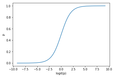
The above expression can be rewritten $g(x)=\frac{1}{1 + e^{-x}}$
It is the function we use to link the structural component of the regression to the response variable.
def logistic(x):
    return 1/(1+np.exp(-x))
plt.plot(logit(p), logistic(p))
plt.ylabel('p')
plt.xlabel('logit(p)');

Using the logistic equation, we would like to build a regression that predict a probability.
A first model could be written as :
$y=\frac{e^{\beta_0 + \beta_1 x}}{1 + e^(\beta_0 + \beta_1 x)}$
where $\beta_0$ and $\beta_1$ have to be estimated.
$y$ is the estimated value we obtain thanks to $\beta_0$ and $\beta_1$. $\beta_0$ is a bias (intercept) and $\beta_1$ is the coefficient associated with x. In this case our model has only one input variable. A model with more than one variable is also possible.
A logistic regression will output probability of a particular class. For instance, if we try to predict whether an animal is a dog (class 1) or a cat (class 0) given its weight, the model output is :
$P(animal = dog|weight)$
The obtained probability can be transformed into binary classification thanks to a threshold (usually 0.5).
In order to work with an easier model, we can transform the equation to have the simplest expression on the right hand side :
$P(X)=\frac{e^{\beta_0 + \beta_1 X}}{1 + e^(\beta_0 + \beta_1 X)}$
$ln(\frac{p(X)}{1 – p(X)}) = \beta_0 + \beta_1 X$
The expression on the right is linear and the expression on the left is the natural logarithm of the odds :
$ln(odds) = \beta_0 + \beta_1 X$
or
$odds = e^{\beta_0 + \beta_1 X}$
2. Making dummy data
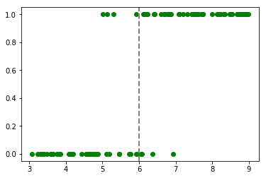
We will generate a dummy dataset on dogs and cats weights. Let’s start by make two perfectly separated classes. Say a cat weights between 3 and 6 kg and a dog weights between 6 and 9 kg :
np.random.seed(26)
obs=np.random.uniform(3, 9, size = 100)
classes = np.where(obs>=6,"dog","cat")
classes_numerical = np.where(classes == "dog", 1, 0)
len(classes_numerical[classes_numerical==1])
54
Our dataset has 54 dogs and 46 cats. To add some noise, some animals weighting between 5 and 7 kg will be assigned to the other class.
mask = (obs>5) & (obs<7) & (classes=="dog")
dogs_eligible_to_change = np.nonzero(mask)
dogs_to_cats = np.random.choice(dogs_eligible_to_change[0], size = 4, replace = False)
classes[dogs_to_cats] = "cat"
mask = (obs>5) & (obs<7) & (classes=="cat")
cats_eligible_to_change = np.nonzero(mask)
cats_to_dogs = np.random.choice(cats_eligible_to_change[0], size = 4, replace = False)
classes[cats_to_dogs] = "dog"
classes_numerical = np.where(classes == "dog", 1, 0)
plt.plot(obs, classes_numerical, "go")
plt.axvline(x=6, linewidth=2, color='grey', linestyle='--');
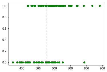
Let’s now make a second variables that describes the yearly budget spent on a pet. Let’s think dogs cost more in average :
dog_budget = 100*np.random.randn(len(classes[classes=="dog"]))+600
cat_budget = 100*np.random.randn(len(classes[classes=="cat"]))+500
budget = np.ones(100)
budget[classes == "dog"] = dog_budget
budget[classes == "cat"] = cat_budget
plt.plot(budget, classes_numerical, "go")
plt.axvline(x=550, linewidth=2, color='grey', linestyle='--');
3. Estimation of the Coefficients
3.1 Stochastic Gradient Descent
To estimate $\beta_0$ and $\beta_1$, the gradient descent algorithm can be used. To start, the stochastic gradient descent will be implemented. The stochastic gradient descent algorithm is a particular case of the gradient descent algorithm. Using the stochastic form will allow us to better visualize the steps in the estimation process.
This algorithm requires two additional parameters :
- The number of epochs. It is the number of times the dataset is read by the algorithm.
- The learning rate. It is the rate used to update our coefficients. If too large, it can miss the minimum, if too small, it could take ages before getting a satisfying result.
The steps of the algorithm :
- Start a new epoch.
- Within this epoch, iterate over each row of the dataset.
- Use a given row to update coefficients.
Here, all rows will be iterated over. In case a dataset is very large, rows can be taken randomly (hence stochastic). This method is particularly useful if the dataset does not hold in memory.
To start, we need to define the log-likelihood function $h_{\theta}$. The algorithm will then try to maximize it.
Let us remember :
$P(y=1|x) = \frac{1}{1 + e^{-\theta^{T}x}}$
And as this is a binary classifier:
$P(y=0|x) = 1- \frac{1}{1 + e^{-\theta^{T}x}}$
$h_{\theta} = \sum_{i=1}^{m} y^{(i)} \log P(y=1) + (1 - y^{(i)}) \log P(y=0)$
Finally :
$h_{\theta} = \sum_{i=1}^{m} y^{(i)} \log \left(\frac{1}{1 + e^{-\theta^{T}x}}\right) + (1 - y^{(i)}) \log \left(1- \frac{1}{1 + e^{-\theta^{T}x}}\right)$
The gradient ascent rule is given by the following expression :
$\theta_{j} := \theta_{j} + \alpha(y^{(i)} - h_{\theta}(x^{(i)})x_{j}^{(i)})$
Please refer to this documentation for all the mathematical details : Stanford Lecture Notes
def predict(weight, coefficients):
    x= coefficients[0] + coefficients[1] * weight
    return 1/(1+np.exp(-x))

def get_coef(weights, target, epochs=100, learning_rate=0.1):
    coef = [0.0, 0.0]
    for epoch in range(epochs):
        sum_error = 0
        for ind, weight in enumerate(weights):
            yhat = predict(weight, coef)
            error = target[ind] - yhat
            sum_error += error**2
            coef[0] = coef[0] + learning_rate * error * yhat * (1.0 - yhat) * 1
            coef[1] = coef[1] + learning_rate * error * yhat * (1.0 - yhat) * weight
        try:
            if (epochs % epoch) == 0 or epoch==epochs-1:
                print("epoch :", epoch,":", "sq. error :", round(sum_error, 2))
        except ZeroDivisionError:
            pass
    return coef
The two most important lines are :
coef[0] = coef[0] + learning_rate * error * yhat * (1.0 - yhat) * 1
coef[1] = coef[1] + learning_rate * error * yhat * (1.0 - yhat) * weight
The first line updates the intercept using the error, the learning rate and the predicted value.
The second line updates the $\beta_1$ coefficient using the error, the learning rate, the predicted value and the weight.
Writing *1 seems useless but it shows the intercept is fitted exacty the same way as the other variables.
calculated_coef = get_coef(obs, classes_numerical, epochs=100)
epoch : 1 : sq. error : 24.22
epoch : 2 : sq. error : 23.08
epoch : 4 : sq. error : 21.02
epoch : 5 : sq. error : 20.11
epoch : 10 : sq. error : 16.61
epoch : 20 : sq. error : 12.96
epoch : 25 : sq. error : 11.97
epoch : 50 : sq. error : 9.73
epoch : 99 : sq. error : 8.5
calculated_coef
[-7.0852236091318419, 1.2644875716003465]
to_predict = np.arange(2, 10, 0.1)
predicted = predict(to_predict, calculated_coef)
plt.plot(obs, classes_numerical, "go")
plt.plot(to_predict, predicted, color='red', linestyle='-')
plt.axvline(x=6, linewidth=2, color='grey', linestyle='--');
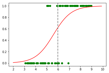
predict(6, calculated_coef)
0.62285918190295297
The result with 100 epochs is not satysfying. Let’s now try with 10 000 epochs :
calculated_coef = get_coef(obs, classes_numerical, epochs=10000)
epoch : 1 : sq. error : 24.22
epoch : 2 : sq. error : 23.08
epoch : 4 : sq. error : 21.02
epoch : 5 : sq. error : 20.11
epoch : 8 : sq. error : 17.82
epoch : 10 : sq. error : 16.61
epoch : 16 : sq. error : 14.06
epoch : 20 : sq. error : 12.96
epoch : 25 : sq. error : 11.97
epoch : 40 : sq. error : 10.32
epoch : 50 : sq. error : 9.73
epoch : 80 : sq. error : 8.81
epoch : 100 : sq. error : 8.49
epoch : 125 : sq. error : 8.23
epoch : 200 : sq. error : 7.84
epoch : 250 : sq. error : 7.71
epoch : 400 : sq. error : 7.51
epoch : 500 : sq. error : 7.44
epoch : 625 : sq. error : 7.39
epoch : 1000 : sq. error : 7.31
epoch : 1250 : sq. error : 7.28
epoch : 2000 : sq. error : 7.24
epoch : 2500 : sq. error : 7.23
epoch : 5000 : sq. error : 7.2
epoch : 9999 : sq. error : 7.18
to_predict = np.arange(2, 10, 0.1)
predicted = predict(to_predict, calculated_coef)
plt.plot(obs, classes_numerical, "go")
plt.plot(to_predict, predicted, color='red', linestyle='-')
plt.axvline(x=6, linewidth=2, color='grey', linestyle='--');
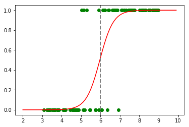
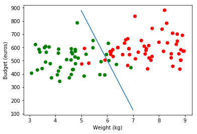
We can now extend this method to a dataset containing more than one variable :
plt.scatter(obs, budget, color=np.where(classes_numerical==1, "red", "green"))
plt.ylabel('Budget (euros)')
plt.xlabel('Weight (kg)')
plt.legend(loc=2);
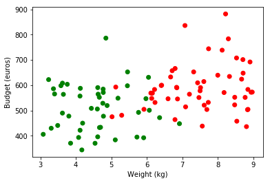
As shown above, our dataset has now two dimensions. Hence, we would like to remake previous calculations taking into account this new coefficient. Let’s rewrite the two functions we need to do so :
def predict_2d(weight, budget, coefficients):
    x = coefficients[0] + coefficients[1] * weight + coefficients[2] * budget
    return 1.0/(1.0+np.exp(-x))

def get_coef_2d(weights, budgets, target, epochs=100, learning_rate=0.1):
    coef = [0.0, 1.0, 1.0]
    for epoch in range(epochs):
        sum_error = 0.0
        for ind, _ in enumerate(weights):
            yhat = predict_2d(weights[ind], budgets[ind], coef)
            error = target[ind] - yhat
            sum_error += error**2
            #print(learning_rate, error, yhat, (1.0 - yhat))
            coef[0] = coef[0] + learning_rate * error * yhat * (1.0 - yhat) * 1
            coef[1] = coef[1] + learning_rate * error * yhat * (1.0 - yhat) * weights[ind]
            coef[2] = coef[2] + learning_rate * error * yhat * (1.0 - yhat) * budgets[ind]
        try:
            if (epochs % epoch) == 0 or epoch==epochs-1:
                print("epoch :", epoch,":", "sq. error :", round(sum_error, 2))
        except ZeroDivisionError:
            pass
    return coef
As an additional step, we scale the buget variable. Why ? Because in this example, if we gave the budget as it is, the yhat variable would be stuck to one and (1.0-yhat) would be stuck to 0. If the expression learning_rate * error * yhat * (1.0 - yhat) * budgets[ind] is 0 the coefficients are not updated. The problem come from the fact that 0.9999999999.. is transformed to 1. The logistic function is never equal to 1.
budget_scaled = (budget - np.mean(budget)) / np.std(budget)
calculated_coef = get_coef_2d(obs, budget_scaled, target = classes_numerical, epochs=1000)
epoch : 1 : sq. error : 19.8
epoch : 2 : sq. error : 19.29
epoch : 4 : sq. error : 18.3
epoch : 5 : sq. error : 17.83
epoch : 8 : sq. error : 16.51
epoch : 10 : sq. error : 15.71
epoch : 20 : sq. error : 12.77
epoch : 25 : sq. error : 11.84
epoch : 40 : sq. error : 10.2
epoch : 50 : sq. error : 9.59
epoch : 100 : sq. error : 8.29
epoch : 125 : sq. error : 8.02
epoch : 200 : sq. error : 7.59
epoch : 250 : sq. error : 7.44
epoch : 500 : sq. error : 7.12
epoch : 999 : sq. error : 6.95
calculated_coef
[-12.574667198935296, 2.1421910360925467, 0.57637784465600761]
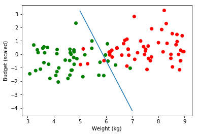
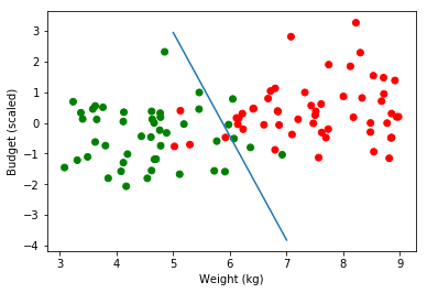
To help visualize, let’s find, for x given, the y needed to get a probability of 0.5 (quick and dirty method) :
def estimate_frontier(calculated_coef):
    for weight in range(5,8):
        x = 0
        for epoch in range(10000):
            if predict_2d(weight, x, calculated_coef) > 0.5:
                x -= 0.01
            else:
                x +=0.01
        print("weight:", weight, "Budget Scaled :", round(x, 2),
              "Estimated Probability", round(predict_2d(weight, x, calculated_coef), 3),
              "Real Budget Value: ", round((x*np.std(budget))+np.mean(budget), 2))
estimate_frontier(calculated_coef)
weight: 5 Budget Scaled : 3.24 Estimated Probability 0.501 Real Budget Value:  879.37
weight: 6 Budget Scaled : -0.48 Estimated Probability 0.5 Real Budget Value:  504.16
weight: 7 Budget Scaled : -4.2 Estimated Probability 0.5 Real Budget Value:  128.95
plt.scatter(obs, budget_scaled, color=np.where(classes_numerical==1, "red", "green"))
plt.plot(range(5,8), [3.24, -0.48, -4.2])
plt.ylabel('Budget (scaled)')
plt.xlabel('Weight (kg)')
plt.legend(loc=2);
On real Budget values :
plt.scatter(obs, budget, color=np.where(classes_numerical==1, "red", "green"))
plt.plot(range(5,8), [879.37, 504.16, 128.95])
plt.ylabel('Budget (euros)')
plt.xlabel('Weight (kg)')
plt.legend(loc=2);
3.2 Gradient Descent
The Gradient Descent is similar to the stochastic Gradient Descent. Instead of looping over each row to adjust coefficients, a loss function is computed taking into account every single row of the dataset. Coefficients are then updated minimizing the error at the dataset level (and not iteratively on the row level). These two methods should converge though.
To start, we need to define the log-likelihood function. The algorithm will then try to maximize it.
Let us define a global loss function :
$h = sigmoid(X\theta)$
$loss = \frac{1}{m}(-y^T log(h)-(1-y)^T log(1-h))$
where $y$ is the target matrix (target in the code below). h is the prediction given the current coefficients (yhat in the code below).
It is exactly the same function we took for the stochastic gradient descent. Minimizing the sum or the mean yields the same results.
The partial derivative of this expression (with respect to coefficients) :
$gradient = \frac{1}{m}X^T(h-y)$
def predict_gd(features, coefficients):
    x = features @ coefficients
    return 1.0/(1.0+np.exp(-x))

def get_coef_gd(features, target, epochs=100, learning_rate=0.1, verbose = False):
    coef = np.zeros(features.shape[1])
    sum_error = 0.0
    if verbose == True:
        print("size of features matrix :", features.shape,
             "\nsize of the target matrix :", target.shape)
    for epoch in range(epochs):
        yhat = predict_gd(features, coef)
        loss = (-target * np.log(yhat) - (1 - target) * np.log(1 - yhat)).mean()
        gradient = np.dot(features.T, (yhat - target)) / target.shape[0]
        coef -= learning_rate * gradient
        try:
            if verbose == True and ((epochs % epoch) == 0 or epoch==epochs-1):
                print("epoch :", epoch,":", "loss function :", round(loss, 2))
                print("gradient :", gradient)
        except ZeroDivisionError:
            pass
    return coef
features = np.zeros(shape = (100, 3))
features[:,0] = 1
features[:,1] = obs
features[:,2] = budget_scaled
features[:10]
array([[ 1.        ,  4.84760972,  2.31483495],
       [ 1.        ,  6.11634888,  0.1599445 ],
       [ 1.        ,  7.60978597,  0.61183027],
       [ 1.        ,  7.73532442, -0.20567959],
       [ 1.        ,  8.22337237,  3.26274692],
       [ 1.        ,  4.12752835,  0.34720225],
       [ 1.        ,  4.61703147, -1.55462483],
       [ 1.        ,  5.97715285, -0.05782319],
       [ 1.        ,  7.43473048,  0.56307285],
       [ 1.        ,  4.16971195, -2.06848982]])
calculated_coef = get_coef_gd(features, target = classes_numerical, epochs=300000, verbose=False)
calculated_coef
array([-14.39080786, 2.45152564, 0.72575361])
estimate_frontier(calculated_coef)
weight: 5 Budget Scaled : 2.94 Estimated Probability 0.5 Real Budget Value:  849.11
weight: 6 Budget Scaled : -0.44 Estimated Probability 0.5 Real Budget Value:  508.2
weight: 7 Budget Scaled : -3.82 Estimated Probability 0.499 Real Budget Value:  167.28
plt.scatter(obs, budget_scaled, color=np.where(classes_numerical==1, "red", "green"))
#plt.plot(range(5,8), [3.24, -0.48, -4.2])
plt.plot(range(5,8), [2.94, -0.44, -3.82])
plt.ylabel('Budget (scaled)')
plt.xlabel('Weight (kg)')
plt.legend(loc=2);
4. Quick Comparaison with sklearn
from sklearn.linear_model import LogisticRegression
model_scikit = LogisticRegression(C = 10000) # C = 10 000 means no regularization
model_scikit.fit(features[:,1:3], classes_numerical)
LogisticRegression(C=10000, class_weight=None, dual=False, fit_intercept=True,
          intercept_scaling=1, max_iter=100, multi_class='ovr', n_jobs=1,
          penalty='l2', random_state=None, solver='liblinear', tol=0.0001,
          verbose=0, warm_start=False)
model_scikit.coef_, model_scikit.intercept_
(array([[ 2.44875396, 0.7254136 ]]), array([-14.37420065]))
preds = model_scikit.predict(features[:,1:3])
# accuracy
(preds == classes_numerical).mean()
0.91000000000000003
Without regularization, we find almost same coefficients.