This short article shows how to estimate a multiple linear regression from scratch. We will use Gradient Descent and compare our results with the results we got from the normal equation (analytical).
Parameter $\beta$ :
$\beta = (X^TX)^{-1} X^T\vec{y}$ where X and y are matrices.
Let’s start by importing packages.
import sys
import numpy as np
import matplotlib.pyplot as plt
%matplotlib inline
import pandas as pd

np.random.seed(123)
We now generate dummy data.
x1, x2 and x3 are random variable we will use to build Y :
x1 = np.random.randn(100)
x2 = np.random.randn(100)
x3 = np.random.randn(100)
Y is defined as a linear relationship between x1, x2 and x3 :
Coefficients can be changed.
Y = 0.2*x1 + 2*x2 + 7*x3 + 1.2
Y = Y + (np.random.randn(100)/1) # adding some noise
Let’s build our matrix X. We add a column of ones np.ones(100) to take the intercept into account. If you don’t want to fit the intercept, you can use [x1, x2, x3] :
FIT_INTERCEPT = True

if FIT_INTERCEPT:
    BigX = np.array([np.ones(100), x1, x2, x3]).T
else:
    BigX = np.array([x1, x2, x3]).T
BigX.shape
(100, 4)
pd.DataFrame(BigX).head(10)
.dataframe tbody tr th {
    vertical-align: top;
}

.dataframe thead th {
    text-align: right;
}
We are now able to compute coefficients thanks to the formula.
Let’s start by the first part of the equation $(X^TX)$..T is used to transpose a matrix and .dot() returns a product of two matrices :
xTx = BigX.T.dot(BigX)
np.linalg is used to compute the inverse of the above expression $(X^TX)^{-1} $ :
XtX = np.linalg.inv(xTx)
And $(X^TX)^{-1} X^T $ :
XtX_xT = XtX.dot(BigX.T)
XtX_xT.shape
(4, 100)
Finally, to get $\beta$, we need to multiply the complete expression by $Y \Rightarrow (X^TX)^{-1} X^T\vec{y}$ :
theta = XtX_xT.dot(Y)
theta
array([1.08557375, 0.11763789, 2.07681273, 7.16222319])
Gradient Descent
To solve a linear regression with Gradient Descent, a cost function is defined. Then, the gradient descent algorithm tries to minimize the cost function by successive iterations :
$loss_{regression} = \frac{1}{N}\sum_{i=1}^n (\hat{y}_n - y_n)^2$
Hence the loss fo a particular point n:
$loss = (\hat{y}_n - y_n)^2$
Each gradient can be obtained taking the partial derivative of the loss function :
$\frac{\partial loss}{\partial \theta_0}$
$\frac{\partial loss}{\partial \theta_1}$
$\frac{\partial loss}{\partial \theta_2}$
$\frac{\partial loss}{\partial \theta_3}$
As $\hat{y}_n = \theta_0 + \theta_1 x_1 + \theta_2 x_2 + \theta_3 x_3 $ the loss for a particular point n can be rewritten :
$loss = (\theta_0 + \theta_1 x_1 + \theta_2 x_2 + \theta_3 x_3 - y_n)^2$
Hence
$\frac{\partial loss}{\partial \theta_1} = 2\theta_1(\theta_0 + \theta_1 x_1 + \theta_2 x_2 + \theta_3 x_3 - y_n)$
To find the final estimation, the algorithm has to iteratively adapt $\theta$ to come closer and closer to the real $\theta$. At the first iteration $\theta$ is chosen randomly.
For each iteration, the algorithm computes $(\hat{y}_n - y_n)$ for each point $n$. Points are stored in a one-column vector $E$.
Each gradient is computed with a matrix operation :
$2X^T E / m$
To help visualise, if your regression has an itercept (like here) the first gradient is equal to $2$ time the sum of all elements in E divided by the number of points. If the gradient is negative, it means $\theta_0$ should be increase in order to minimize the loss function. If the gradient is positive, we should decrease $\theta_0$ in order to minimize the loss function.
To update $\theta$, a learning rate is used to adjust the speed of learning :
$\theta = \theta - \sigma * gradients$
where $\theta$ and $gradients$ are one-column vectors.
First, we define some parameters for our gradient :
eta is the learning rate, n_iter is the number of iterations and m is the number of data points :
eta = 0.1
n_iter = 100
m=100
theta2 = np.random.randn(4,1)
theta2_before = theta2[0][0].copy()
theta2
array([[ 1.53409029],
       [-0.5299141 ],
       [-0.49097228],
       [-1.30916531]])
diff = BigX @ theta2 - Y[:, np.newaxis]
gradient = 2/m * (BigX.T @ diff)
theta2 = theta2 - eta * gradient
theta2_after = theta2_before - eta * gradient[0][0]
theta2_after - theta2_before
-0.25740388405348535
cost_evo = np.empty(n_iter)
for i in range(n_iter):
    diff = BigX @ theta2 - Y[:, np.newaxis]
    gradient = 2/m * (BigX.T @ diff)
    theta2 = theta2 - eta * gradient
    #
    cost_evo[i] = (diff**2 / m).sum()
theta2
array([[1.08557374],
       [0.11763789],
       [2.07681273],
       [7.16222317]])
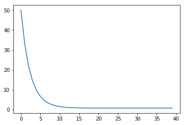
plt.plot(cost_evo[:40]);
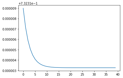
plt.plot(cost_evo[40:80]);
theta2
array([[1.08557374],
       [0.11763789],
       [2.07681273],
       [7.16222317]])
theta
array([1.08557375, 0.11763789, 2.07681273, 7.16222319])
Shorter version :
theta3 = np.random.randn(4,1)
for iteration in range(n_iter):
    gradients = 2/m * BigX.T.dot(BigX.dot(theta3) - Y[:, np.newaxis])
    theta3 = theta3 - eta * gradients
    #
theta3
array([[1.08557373],
       [0.11763789],
       [2.07681273],
       [7.16222316]])
gradients
array([[-4.16419993e-08],
       [-7.12792565e-09],
       [ 1.92325412e-09],
       [-5.84652023e-08]])
theta2-theta3
array([[ 2.10499107e-09],
       [ 3.06503462e-10],
       [-1.15526833e-09],
       [ 3.11118509e-09]])
Coefficients we found thanks to the Gradient Descent Algorithm are very close to Coefficients from the analytical solution. 😄